天池新闻推荐——数据分析
数据分析
数据分析是解决一个数据科学问题的第一步。通过数据可视化 观察数据,再根据情况进行数据预处理 对数据进行清洗。 > 解决数据科学问题的步骤:(源于大佬分享及自己的总结补充) * 数据可视化(观察数据) * 数据预处理(对数据进行清洗) * 文献等资料查阅解决问题的已有方式 * 建立模型,确定目标对象 * 特征工程 * 模型尝试(统计模型、树模型、神经网络) * 特征筛选 * 模型超参数调优 * 交叉验证与模型融合
数据观察与数据分析
导入包
1
2
3
4
5
6
7
8
9
10
%matplotlib inline import pandas as pdimport numpy as npimport matplotlib.pyplot as pltimport seaborn as snsplt.rc('font' , family='SimHei' , size=13 ) import os, gc, re, warnings, syswarnings.filterwarnings('ignore' )
读取数据
1 2 3 4 5 6 7 8 9 path = './raw_data/' trn_click = pd.read_csv(path+'train_click_log.csv' ) item_df = pd.read_csv(path+'articles.csv' ) item_df = item_df.rename(columns={'article_id' : 'click_article_id' }) item_emb_df = pd.read_csv(path+'articles_emb.csv' ) tst_click = pd.read_csv(path+'testA_click_log.csv' )
数据预处理
对每个用户根据用户点击的时间戳进行排序,增加rank列
计算每个用户点击文章的次数(也就是点击时间戳的数量),增加click_cnts列
1 2 3 4 5 trn_click['rank' ] = trn_click.groupby(['user_id' ])['click_timestamp' ].rank(ascending=False ).astype(int ) tst_click['rank' ] = tst_click.groupby(['user_id' ])['click_timestamp' ].rank(ascending=False ).astype(int ) trn_click['click_cnts' ] = trn_click.groupby(['user_id' ])['click_timestamp' ].transform('count' ) tst_click['click_cnts' ] = tst_click.groupby(['user_id' ])['click_timestamp' ].transform('count' )
观察数据
训练集数据:用户点击文章的日志文件
查看时将用户点击文章的数据表和文章数据表根据article_id拼接
1
2
trn_click = trn_click.merge(item_df, how='left' , on=['click_article_id' ]) trn_click.head()
user_id
click_article_id
click_timestamp
click_environment
click_deviceGroup
click_os
click_country
click_region
click_referrer_type
rank
click_cnts
category_id
created_at_ts
words_count
0
199999
160417
1507029570190
4
1
17
1
13
1
11
11
281
1506942089000
173
1
199999
5408
1507029571478
4
1
17
1
13
1
10
11
4
1506994257000
118
2
199999
50823
1507029601478
4
1
17
1
13
1
9
11
99
1507013614000
213
3
199998
157770
1507029532200
4
1
17
1
25
5
40
40
281
1506983935000
201
4
199998
96613
1507029671831
4
1
17
1
25
5
39
40
209
1506938444000
185
<class 'pandas.core.frame.DataFrame'>
Int64Index: 1112623 entries, 0 to 1112622
Data columns (total 14 columns):
user_id                1112623 non-null int64
click_article_id       1112623 non-null int64
click_timestamp        1112623 non-null int64
click_environment      1112623 non-null int64
click_deviceGroup      1112623 non-null int64
click_os               1112623 non-null int64
click_country          1112623 non-null int64
click_region           1112623 non-null int64
click_referrer_type    1112623 non-null int64
rank                   1112623 non-null int64
click_cnts             1112623 non-null int64
category_id            1112623 non-null int64
created_at_ts          1112623 non-null int64
words_count            1112623 non-null int64
dtypes: int64(14)
memory usage: 127.3 MB
user_id
click_article_id
click_timestamp
click_environment
click_deviceGroup
click_os
click_country
click_region
click_referrer_type
rank
click_cnts
category_id
created_at_ts
words_count
count
1.112623e+06
1.112623e+06
1.112623e+06
1.112623e+06
1.112623e+06
1.112623e+06
1.112623e+06
1.112623e+06
1.112623e+06
1.112623e+06
1.112623e+06
1.112623e+06
1.112623e+06
1.112623e+06
mean
1.221198e+05
1.951541e+05
1.507588e+12
3.947786e+00
1.815981e+00
1.301976e+01
1.310776e+00
1.813587e+01
1.910063e+00
7.118518e+00
1.323704e+01
3.056176e+02
1.506598e+12
2.011981e+02
std
5.540349e+04
9.292286e+04
3.363466e+08
3.276715e-01
1.035170e+00
6.967844e+00
1.618264e+00
7.105832e+00
1.220012e+00
1.016095e+01
1.631503e+01
1.155791e+02
8.343066e+09
5.223881e+01
min
0.000000e+00
3.000000e+00
1.507030e+12
1.000000e+00
1.000000e+00
2.000000e+00
1.000000e+00
1.000000e+00
1.000000e+00
1.000000e+00
2.000000e+00
1.000000e+00
1.166573e+12
0.000000e+00
25%
7.934700e+04
1.239090e+05
1.507297e+12
4.000000e+00
1.000000e+00
2.000000e+00
1.000000e+00
1.300000e+01
1.000000e+00
2.000000e+00
4.000000e+00
2.500000e+02
1.507220e+12
1.700000e+02
50%
1.309670e+05
2.038900e+05
1.507596e+12
4.000000e+00
1.000000e+00
1.700000e+01
1.000000e+00
2.100000e+01
2.000000e+00
4.000000e+00
8.000000e+00
3.280000e+02
1.507553e+12
1.970000e+02
75%
1.704010e+05
2.777120e+05
1.507841e+12
4.000000e+00
3.000000e+00
1.700000e+01
1.000000e+00
2.500000e+01
2.000000e+00
8.000000e+00
1.600000e+01
4.100000e+02
1.507756e+12
2.280000e+02
max
1.999990e+05
3.640460e+05
1.510603e+12
4.000000e+00
5.000000e+00
2.000000e+01
1.100000e+01
2.800000e+01
7.000000e+00
2.410000e+02
2.410000e+02
4.600000e+02
1.510666e+12
6.690000e+03
1 2 trn_click.user_id.nunique()
2000001 2 trn_click.groupby(['user_id' ])['click_article_id' ].count().min ()
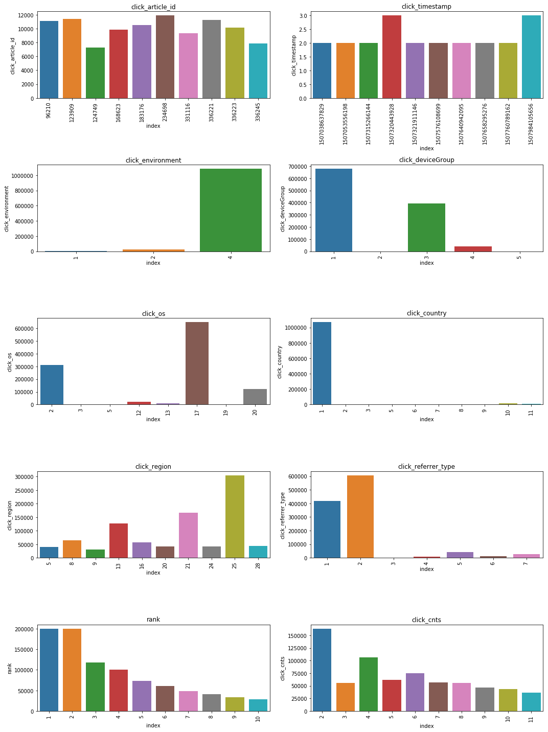
2通过直方图观察用户点击日志文件的各列数据分布
1 2 3 4 5 6 7 8 9 10 11 12 13 14 plt.figure() plt.figure(figsize=(15 , 20 )) i = 1 for col in ['click_article_id' , 'click_timestamp' , 'click_environment' , 'click_deviceGroup' , 'click_os' , 'click_country' , 'click_region' , 'click_referrer_type' , 'rank' , 'click_cnts' ]: plot_envs = plt.subplot(5 , 2 , i) i += 1 v = trn_click[col].value_counts().reset_index()[:10 ] fig = sns.barplot(x=v['index' ], y=v[col]) for item in fig.get_xticklabels(): f=item.set_rotation(90 ) plt.title(col) plt.tight_layout() plt.show()
<Figure size 432x288 with 0 Axes>
png
分析 * 从点击时间clik_timestamp来看,分布较为平均,可不做特殊处理。由于时间戳是13位的,后续将时间格式转换成10位方便计算。
测试集用户点击日志
1 2 tst_click = tst_click.merge(item_df, how='left' , on=['click_article_id' ]) tst_click.head()
user_id
click_article_id
click_timestamp
click_environment
click_deviceGroup
click_os
click_country
click_region
click_referrer_type
rank
click_cnts
category_id
created_at_ts
words_count
0
249999
160974
1506959142820
4
1
17
1
13
2
19
19
281
1506912747000
259
1
249999
160417
1506959172820
4
1
17
1
13
2
18
19
281
1506942089000
173
2
249998
160974
1506959056066
4
1
12
1
13
2
5
5
281
1506912747000
259
3
249998
202557
1506959086066
4
1
12
1
13
2
4
5
327
1506938401000
219
4
249997
183665
1506959088613
4
1
17
1
15
5
7
7
301
1500895686000
256
user_id
click_article_id
click_timestamp
click_environment
click_deviceGroup
click_os
click_country
click_region
click_referrer_type
rank
click_cnts
category_id
created_at_ts
words_count
count
518010.000000
518010.000000
5.180100e+05
518010.000000
518010.000000
518010.000000
518010.000000
518010.000000
518010.000000
518010.000000
518010.000000
518010.000000
5.180100e+05
518010.000000
mean
227342.428169
193803.792550
1.507387e+12
3.947300
1.738285
13.628467
1.348209
18.250250
1.819614
15.521785
30.043586
305.324961
1.506883e+12
210.966331
std
14613.907188
88279.388177
3.706127e+08
0.323916
1.020858
6.625564
1.703524
7.060798
1.082657
33.957702
56.868021
110.411513
5.816668e+09
83.040065
min
200000.000000
137.000000
1.506959e+12
1.000000
1.000000
2.000000
1.000000
1.000000
1.000000
1.000000
1.000000
1.000000
1.265812e+12
0.000000
25%
214926.000000
128551.000000
1.507026e+12
4.000000
1.000000
12.000000
1.000000
13.000000
1.000000
4.000000
10.000000
252.000000
1.506970e+12
176.000000
50%
229109.000000
199197.000000
1.507308e+12
4.000000
1.000000
17.000000
1.000000
21.000000
2.000000
8.000000
19.000000
323.000000
1.507249e+12
199.000000
75%
240182.000000
272143.000000
1.507666e+12
4.000000
3.000000
17.000000
1.000000
25.000000
2.000000
18.000000
35.000000
399.000000
1.507630e+12
232.000000
max
249999.000000
364043.000000
1.508832e+12
4.000000
5.000000
20.000000
11.000000
28.000000
7.000000
938.000000
938.000000
460.000000
1.509949e+12
3082.000000
训练集和测试集的用户是完全不一样的,训练集的用户ID由0 ~ 199999,而测试集A的用户ID由200000 ~ 249999。
1 2 tst_click.user_id.nunique()
500001 tst_click.groupby('user_id' )['click_article_id' ].count().min ()
1新闻文章信息数据表
1 2 item_df.head().append(item_df.tail())
click_article_id
category_id
created_at_ts
words_count
0
0
0
1513144419000
168
1
1
1
1405341936000
189
2
2
1
1408667706000
250
3
3
1
1408468313000
230
4
4
1
1407071171000
162
364042
364042
460
1434034118000
144
364043
364043
460
1434148472000
463
364044
364044
460
1457974279000
177
364045
364045
460
1515964737000
126
364046
364046
460
1505811330000
479
1 item_df['words_count' ].value_counts()
176 3485
182 3480
179 3463
178 3458
174 3456
183 3432
184 3427
173 3414
180 3403
177 3391
170 3387
187 3355
169 3352
185 3348
175 3346
181 3330
186 3328
189 3327
171 3327
172 3322
165 3308
188 3288
167 3269
190 3261
192 3257
168 3248
193 3225
166 3199
191 3182
194 3164
...
601 1
857 1
1977 1
1626 1
697 1
1720 1
696 1
706 1
592 1
1605 1
586 1
582 1
1606 1
972 1
716 1
584 1
1608 1
715 1
841 1
968 1
964 1
587 1
1099 1
1355 1
711 1
845 1
710 1
965 1
847 1
1535 1
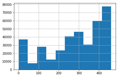
Name: words_count, Length: 866, dtype: int641 2 print(item_df['category_id' ].nunique()) item_df['category_id' ].hist()
461
<matplotlib.axes._subplots.AxesSubplot at 0x7f92a1e03080>
png
(364047, 4)新闻文章embedding向量表示
article_id
emb_0
emb_1
emb_2
emb_3
emb_4
emb_5
emb_6
emb_7
emb_8
...
emb_240
emb_241
emb_242
emb_243
emb_244
emb_245
emb_246
emb_247
emb_248
emb_249
0
0
-0.161183
-0.957233
-0.137944
0.050855
0.830055
0.901365
-0.335148
-0.559561
-0.500603
...
0.321248
0.313999
0.636412
0.169179
0.540524
-0.813182
0.286870
-0.231686
0.597416
0.409623
1
1
-0.523216
-0.974058
0.738608
0.155234
0.626294
0.485297
-0.715657
-0.897996
-0.359747
...
-0.487843
0.823124
0.412688
-0.338654
0.320786
0.588643
-0.594137
0.182828
0.397090
-0.834364
2
2
-0.619619
-0.972960
-0.207360
-0.128861
0.044748
-0.387535
-0.730477
-0.066126
-0.754899
...
0.454756
0.473184
0.377866
-0.863887
-0.383365
0.137721
-0.810877
-0.447580
0.805932
-0.285284
3
3
-0.740843
-0.975749
0.391698
0.641738
-0.268645
0.191745
-0.825593
-0.710591
-0.040099
...
0.271535
0.036040
0.480029
-0.763173
0.022627
0.565165
-0.910286
-0.537838
0.243541
-0.885329
4
4
-0.279052
-0.972315
0.685374
0.113056
0.238315
0.271913
-0.568816
0.341194
-0.600554
...
0.238286
0.809268
0.427521
-0.615932
-0.503697
0.614450
-0.917760
-0.424061
0.185484
-0.580292
5 rows × 251 columns
(364047, 251)数据分析
用户重复点击
1 2 user_click_merge = trn_click.append(tst_click)
1 2 3 user_click_count = user_click_merge.groupby(['user_id' , 'click_article_id' ])['click_timestamp' ].agg({'count' }).reset_index() user_click_count[:10 ]
user_id
click_article_id
count
0
0
30760
1
1
0
157507
1
2
1
63746
1
3
1
289197
1
4
2
36162
1
5
2
168401
1
6
3
36162
1
7
3
50644
1
8
4
39894
1
9
4
42567
1
1 user_click_count[user_click_count['count' ]>7 ]
user_id
click_article_id
count
311242
86295
74254
10
311243
86295
76268
10
393761
103237
205948
10
393763
103237
235689
10
576902
134850
69463
13
1 user_click_count['count' ].unique()
array([ 1, 2, 4, 3, 6, 5, 10, 7, 13])1 2 user_click_count.loc[:,'count' ].value_counts()
1 1605541
2 11621
3 422
4 77
5 26
6 12
10 4
7 3
13 1
Name: count, dtype: int64可以看出:有1605541(约占99.2%)的用户未重复阅读过文章,仅有极少数用户重复点击过某篇文章。 这个也可以单独制作成特征
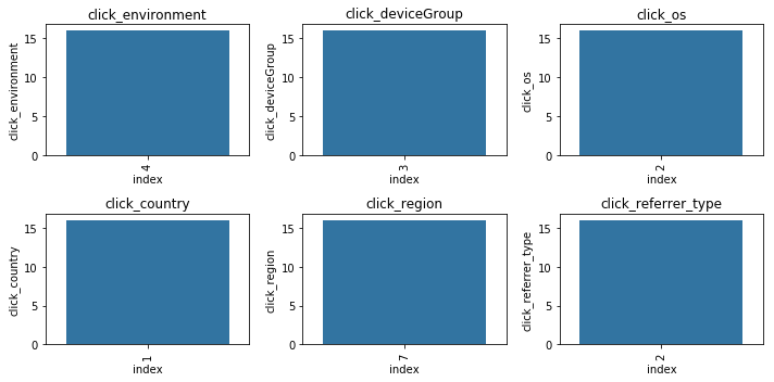
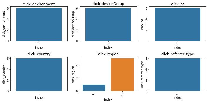
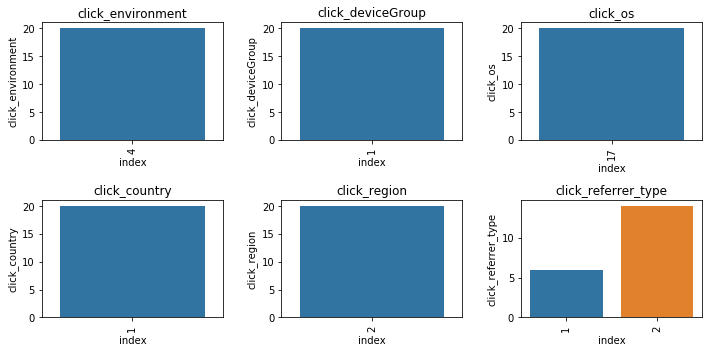
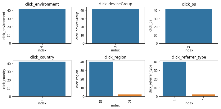
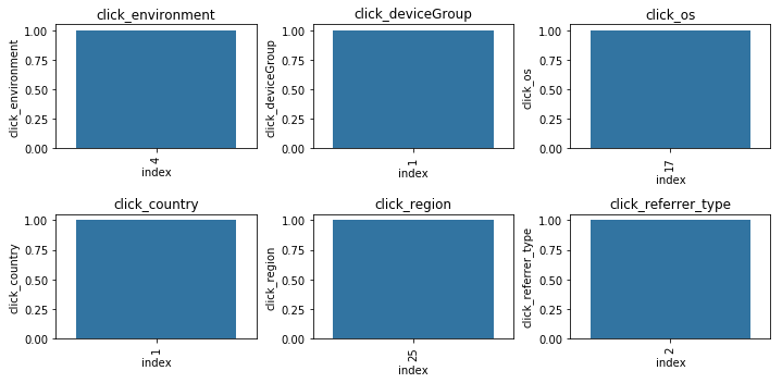
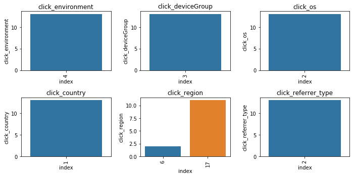
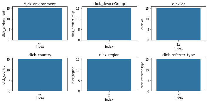
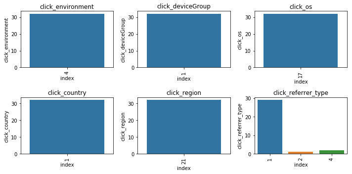
用户点击环境变化分析
1 2 3 4 5 6 7 8 9 10 11 12 13 14 def plot_envs (df, cols, r, c ): plt.figure() plt.figure(figsize=(10 , 5 )) i = 1 for col in cols: plt.subplot(r, c, i) i += 1 v = df[col].value_counts().reset_index() fig = sns.barplot(x=v['index' ], y=v[col]) for item in fig.get_xticklabels(): item.set_rotation(90 ) plt.title(col) plt.tight_layout() plt.show()
1 2 3 4 5 6 sample_user_ids = np.random.choice(tst_click['user_id' ].unique(), size=10 , replace=False ) sample_users = user_click_merge[user_click_merge['user_id' ].isin(sample_user_ids)] cols = ['click_environment' ,'click_deviceGroup' , 'click_os' , 'click_country' , 'click_region' ,'click_referrer_type' ] for _, user_df in sample_users.groupby('user_id' ): plot_envs(user_df, cols, 2 , 3 )
<Figure size 432x288 with 0 Axes>
png
<Figure size 432x288 with 0 Axes>
png
<Figure size 432x288 with 0 Axes>
png
<Figure size 432x288 with 0 Axes>
png
<Figure size 432x288 with 0 Axes>
png
<Figure size 432x288 with 0 Axes>
png
<Figure size 432x288 with 0 Axes>
png
<Figure size 432x288 with 0 Axes>
png
<Figure size 432x288 with 0 Axes>
png
<Figure size 432x288 with 0 Axes>
png
可以看出绝大多数数的用户的点击环境是比较固定的。思路:可以基于这些环境的统计特征来代表该用户本身的属性
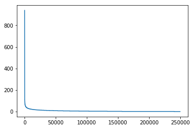
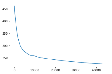
用户点击新闻数量的分布
1 2 user_click_item_count = sorted (user_click_merge.groupby('user_id' )['click_article_id' ].count(), reverse=True ) plt.plot(user_click_item_count)
[<matplotlib.lines.Line2D at 0x7f92a03e6cf8>]
png
可以根据用户的点击文章次数看出用户的活跃度
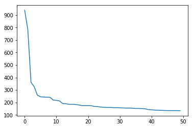
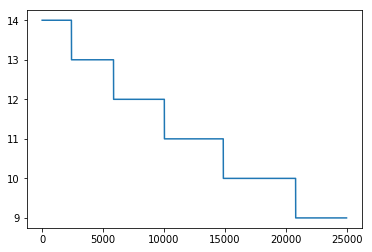
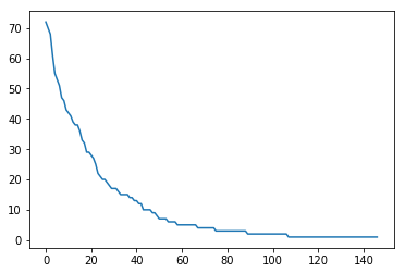
1 2 plt.plot(user_click_item_count[:50 ])
[<matplotlib.lines.Line2D at 0x7f92a0391ba8>]
png
点击次数排前50的用户的点击次数都在100次以上。思路:我们可以定义点击次数大于等于100次的用户为活跃用户,这是一种简单的处理思路, 判断用户活跃度,更加全面的是再结合上点击时间,后面我们会基于点击次数和点击时间两个方面来判断用户活跃度。
1 2 plt.plot(user_click_item_count[25000 :50000 ])
[<matplotlib.lines.Line2D at 0x7f92a04d3240>]
png
可以看出点击次数小于等于两次的用户非常的多,这些用户可以认为是非活跃用户。
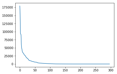
新闻点击次数分析
1 item_click_count = sorted (user_click_merge.groupby('click_article_id' )['user_id' ].count(), reverse=True )
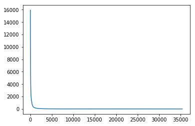
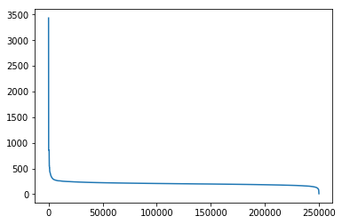
1 plt.plot(item_click_count)
[<matplotlib.lines.Line2D at 0x7f92a014c4a8>]
png
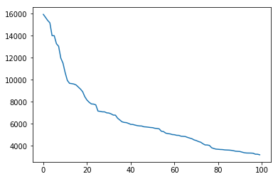
1 plt.plot(item_click_count[:100 ])
[<matplotlib.lines.Line2D at 0x7f92a1a04eb8>]
png
可以看出点击次数最多的前100篇新闻,点击次数大于1000次
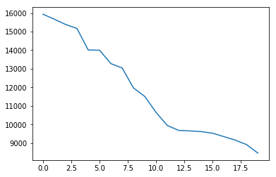
1 plt.plot(item_click_count[:20 ])
[<matplotlib.lines.Line2D at 0x7f92a1ad99e8>]
png
点击次数最多的前20篇新闻,点击次数大于2500。思路:可以定义这些新闻为热门新闻, 这个也是简单的处理方式,后面我们也是根据点击次数和时间进行文章热度的一个划分。
1 plt.plot(item_click_count[3500 :])
[<matplotlib.lines.Line2D at 0x7f92a1c82208>]
png
可以发现很多新闻只被点击过一两次。思路:可以定义这些新闻是冷门新闻
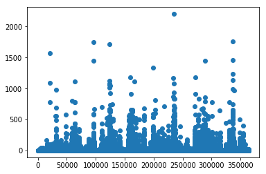
新闻共现频次:两篇新闻连续出现的次数
1 2 3 4 tmp = user_click_merge.sort_values('click_timestamp' ) tmp['next_item' ] = tmp.groupby(['user_id' ])['click_article_id' ].transform(lambda x:x.shift(-1 )) union_item = tmp.groupby(['click_article_id' ,'next_item' ])['click_timestamp' ].agg({'count' }).reset_index().sort_values('count' , ascending=False ) union_item[['count' ]].describe()
count
count
433597.000000
mean
3.184139
std
18.851753
min
1.000000
25%
1.000000
50%
1.000000
75%
2.000000
max
2202.000000
由统计数据可以看出,平均共现次数2.88,最高为1687。
说明用户看的新闻,相关性是比较强的。
1 2 3 4 x = union_item['click_article_id' ] y = union_item['count' ] plt.scatter(x, y)
<matplotlib.collections.PathCollection at 0x7f92a033cdd8>
png
1 plt.plot(union_item['count' ].values[40000 :])
[<matplotlib.lines.Line2D at 0x7f92a0477d68>]
png
大概有70000个pair至少共现一次
新闻文章信息
1 2 plt.plot(user_click_merge['category_id' ].value_counts().values)
[<matplotlib.lines.Line2D at 0x7f92a02d1c50>]
png
1 2 plt.plot(user_click_merge['category_id' ].value_counts().values[150 :])
[<matplotlib.lines.Line2D at 0x7f9295dcdf28>]
png
1 2 user_click_merge['words_count' ].describe()
count 1.630633e+06
mean 2.043012e+02
std 6.382198e+01
min 0.000000e+00
25% 1.720000e+02
50% 1.970000e+02
75% 2.290000e+02
max 6.690000e+03
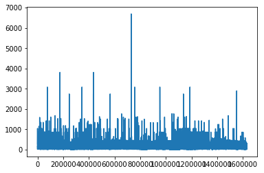
Name: words_count, dtype: float641 plt.plot(user_click_merge['words_count' ].values)
[<matplotlib.lines.Line2D at 0x7f92a02c2390>]
png
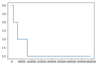
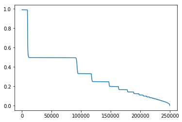
用户点击的新闻类型的偏好
此特征可以用于度量用户的兴趣是否广泛。
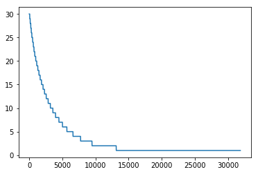
1 plt.plot(sorted (user_click_merge.groupby('user_id' )['category_id' ].nunique(), reverse=True ))
[<matplotlib.lines.Line2D at 0x7f92a0283cc0>]
png
可以看出有一小部分用户阅读类型是极其广泛的,大部分人都处在20个新闻类型以下。
1 user_click_merge.groupby('user_id' )['category_id' ].nunique().reset_index().describe()
user_id
category_id
count
250000.000000
250000.000000
mean
124999.500000
4.573188
std
72168.927986
4.419800
min
0.000000
1.000000
25%
62499.750000
2.000000
50%
124999.500000
3.000000
75%
187499.250000
6.000000
max
249999.000000
95.000000
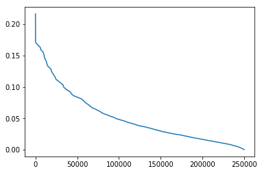
用户查看文章的长度的分布
通过统计不同用户点击新闻的平均字数,这个可以反映用户是对长文更感兴趣还是对短文更感兴趣。
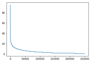
1 plt.plot(sorted (user_click_merge.groupby('user_id' )['words_count' ].mean(), reverse=True ))
[<matplotlib.lines.Line2D at 0x7f9294f8c9b0>]
png
可以发现有一小部分人看的文章平均词数非常高,也有一小部分人看的平均文章次数非常低。
大多数人偏好于阅读字数在200-400字之间的新闻。
1 2 plt.plot(sorted (user_click_merge.groupby('user_id' )['words_count' ].mean(), reverse=True )[1000 :45000 ])
[<matplotlib.lines.Line2D at 0x7f925a255f98>]
png
可以发现大多数人都是看250字以下的文章
1 2 user_click_merge.groupby('user_id' )['words_count' ].mean().reset_index().describe()
user_id
words_count
count
250000.000000
250000.000000
mean
124999.500000
205.830189
std
72168.927986
47.174030
min
0.000000
8.000000
25%
62499.750000
187.500000
50%
124999.500000
202.000000
75%
187499.250000
217.750000
max
249999.000000
3434.500000
用户点击新闻的时间分析
1 2 3 4 5 6 7 from sklearn.preprocessing import MinMaxScalermm = MinMaxScaler() user_click_merge['click_timestamp' ] = mm.fit_transform(user_click_merge[['click_timestamp' ]]) user_click_merge['created_at_ts' ] = mm.fit_transform(user_click_merge[['created_at_ts' ]]) user_click_merge = user_click_merge.sort_values('click_timestamp' )
user_id
click_article_id
click_timestamp
click_environment
click_deviceGroup
click_os
click_country
click_region
click_referrer_type
rank
click_cnts
category_id
created_at_ts
words_count
18
249990
162300
0.000000
4
3
20
1
25
2
5
5
281
0.989186
193
2
249998
160974
0.000002
4
1
12
1
13
2
5
5
281
0.989092
259
30
249985
160974
0.000003
4
1
17
1
8
2
8
8
281
0.989092
259
50
249979
162300
0.000004
4
1
17
1
25
2
2
2
281
0.989186
193
25
249988
160974
0.000004
4
1
17
1
21
2
17
17
281
0.989092
259
1 2 3 4 5 def mean_diff_time_func (df, col ): df = pd.DataFrame(df, columns={col}) df['time_shift1' ] = df[col].shift(1 ).fillna(0 ) df['diff_time' ] = abs (df[col] - df['time_shift1' ]) return df['diff_time' ].mean()
1 2 mean_diff_click_time = user_click_merge.groupby('user_id' )['click_timestamp' , 'created_at_ts' ].apply(lambda x: mean_diff_time_func(x, 'click_timestamp' ))
1 plt.plot(sorted (mean_diff_click_time.values, reverse=True ))
[<matplotlib.lines.Line2D at 0x7f929880f4e0>]
png
可以发现不同用户点击文章的时间差是有差异的。
1 2 mean_diff_created_time = user_click_merge.groupby('user_id' )['click_timestamp' , 'created_at_ts' ].apply(lambda x: mean_diff_time_func(x, 'created_at_ts' ))
1 plt.plot(sorted (mean_diff_created_time.values, reverse=True ))
[<matplotlib.lines.Line2D at 0x7f9298758fd0>]
png
可以发现用户先后点击文章,文章的创建时间也是有差异的
1 2 item_idx_2_rawid_dict = dict (zip (item_emb_df['article_id' ], item_emb_df.index))
1 del item_emb_df['article_id' ]
1 item_emb_np = np.ascontiguousarray(item_emb_df.values, dtype=np.float32)
1 2 3 4 5 sub_user_ids = np.random.choice(user_click_merge.user_id.unique(), size=15 , replace=False ) sub_user_info = user_click_merge[user_click_merge['user_id' ].isin(sub_user_ids)] sub_user_info.head()
user_id
click_article_id
click_timestamp
click_environment
click_deviceGroup
click_os
click_country
click_region
click_referrer_type
rank
click_cnts
category_id
created_at_ts
words_count
69935
223960
272143
0.005832
4
3
20
6
28
2
4
4
399
0.989235
184
69936
223960
160974
0.005852
4
3
20
6
28
1
3
4
281
0.989092
259
69937
223960
337082
0.005860
4
3
20
6
28
1
2
4
437
0.989214
163
75534
221873
166581
0.006673
4
1
17
1
25
2
9
9
289
0.989241
210
75535
221873
64329
0.006680
4
1
17
1
25
2
8
9
134
0.989259
199
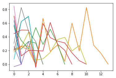
1 2 3 4 5 6 7 8 9 def get_item_sim_list (df ): sim_list = [] item_list = df['click_article_id' ].values for i in range (0 , len (item_list)-1 ): emb1 = item_emb_np[item_idx_2_rawid_dict[item_list[i]]] emb2 = item_emb_np[item_idx_2_rawid_dict[item_list[i+1 ]]] sim_list.append(np.dot(emb1,emb2)/(np.linalg.norm(emb1)*(np.linalg.norm(emb2)))) sim_list.append(0 ) return sim_list
1 2 3 for _, user_df in sub_user_info.groupby('user_id' ): item_sim_list = get_item_sim_list(user_df) plt.plot(item_sim_list)
png
可以看出有些用户前后看的商品的相似度波动比较大,有些波动比较小,也是有一定的区分度的。
总结
训练集和测试集的用户id没有重复,也就是测试集里面的用户模型是没有见过的
训练集中用户最少的点击文章数是2, 而测试集里面用户最少的点击文章数是1
用户对于文章存在重复点击的情况, 但这个都存在于训练集里面
同一用户的点击环境存在不唯一的情况,后面做这部分特征的时候可以采用统计特征
用户点击文章的次数有很大的区分度,后面可以根据这个制作衡量用户活跃度的特征
文章被用户点击的次数也有很大的区分度,后面可以根据这个制作衡量文章热度的特征
用户看的新闻,相关性是比较强的,所以往往我们判断用户是否对某篇文章感兴趣的时候, 在很大程度上会和他历史点击过的文章有关
用户点击的文章字数有比较大的区别, 这个可以反映用户对于文章字数的区别
用户点击过的文章主题也有很大的区别, 这个可以反映用户的主题偏好
不同用户点击文章的时间差也会有所区别, 这个可以反映用户对于文章时效性的偏好