集成学习之Stacking

前面已经了解了Bagging博客传送门和Boosting博客传送门,这篇博客要接着来看集成学习的Stacking

Stacking集成学习严格来说并不是一种算法,而是一种复杂的对模型集成的策略

Stacking集成学习可以理解为两层架构:第一层含有多个基础分类器,把预测的结果(或者称为元特征)传递给第二层;第二层通常拥有一个分类器(一般是逻辑回归),把第一层分类器的结果当作特征进行拟合,最后输出预测结果。基于Stacking进行训练和测试过程如下图所示:

1 Blending

在正式看Stacking之前,先来了解“简化版的Stacking”,也就是Blending

  • 1.1 Blending集成学习的方法和步骤

Blending集成学习的方法和步骤如下:

  1. 将数据划分为原训练集和测试集。其中,原训练集需要再继续划分出训练集和验证集。
  2. 创建第一层的模型。第一层的模型之间可以同质(相同种类)也可以异质(不同种类)。
  3. 使用训练集中的数据来训练第一层的模型(多个);然后将验证集中的数据输入到第一层训练好的模型中得到第一层的预测值。
  4. 创建第二层的模型,使用上一步得到的预测值作为训练集来训练第二层的模型。
  5. 最后将测试集输入第一层模型得到第一层的预测值,然后将第一层的预测值作为输入传递给第二层模型,第二层模型得到的预测结果就是该测试集最终的预测结果。
  • 1.2 对上面Blending的方法和步骤的解释

第1步中数据集最终被分为训练集、验证集以及测试集。一般的步骤是先将数据集中的80%数据划分为训练集,20%的数据划分为测试集;然后,训练集中需要再划分出70%为最终的训练集,30%为验证集。

训练集是用于训练模型参数;验证集是用于调整模型参数;测试集适用于检验模型的效果(是否能够很好地分类或回归)。

第2步是选择第一层的模型。第一层可以选择多个模型,例如K个(K为整数),例如SVM、随机森林、XGBoost等。

第3步就是利用训练集对第一层的各个模型进行训练,然后用训练好的模型对验证集进行预测得到第一层的输出,这里的输出是第一层中K个模型的输出组成的。

关于第一层的输出进行举例:如果总的样本数有10000条,使用了5600个样本训练了第一层的K个模型,输入2400个验证集样本到第一层的K个模型会得到K组2400个预测结果。输入2000个测试集样本到第一层模型会得到K组2000个预测结果。

第4步就是使用第一层各个模型的验证集结果作为第二层分类器的特征训练第二层分类器。

第5步就是将第一层各个模型的测试集结果输入到第二层分类器中得到最终的预测结果。

  • 1.3 Blending案例

加载相关工具包:

1
2
3
4
5
6
7
8
9
10
11
12
13
14
import numpy as np
import pandas as pd
import matplotlib.pyplot as plt
plt.style.use("ggplot")
%matplotlib inline
import seaborn as sns
from sklearn import datasets
from sklearn.datasets import make_blobs
from sklearn.model_selection import train_test_split
from sklearn.svm import SVC
from sklearn.ensemble import RandomForestClassifier
from sklearn.neighbors import KNeighborsClassifier
from sklearn.linear_model import LogisticRegression
from sklearn.model_selection import cross_val_score

创建数据:

1
2
3
4
5
6
7
8
9
10
11
data, target = make_blobs(n_samples=10000, centers=2, random_state=1, cluster_std=1.0 )
## 创建训练集和测试集
X_train1,X_test,y_train1,y_test = train_test_split(data, target, test_size=0.2, random_state=1)
## 创建训练集和验证集
X_train,X_val,y_train,y_val = train_test_split(X_train1, y_train1, test_size=0.3, random_state=1)
print("The shape of training X:",X_train.shape)
print("The shape of training y:",y_train.shape)
print("The shape of validation X:",X_val.shape)
print("The shape of validation y:",y_val.shape)
print("The shape of test X:",X_test.shape)
print("The shape of test y:",y_test.shape)

输出为:

1
2
3
4
5
6
The shape of training X: (5600, 2)
The shape of training y: (5600,)
The shape of validation X: (2400, 2)
The shape of validation y: (2400,)
The shape of test X: (2000, 2)
The shape of test y: (2000,)
创建第一、二层模型:

1
2
3
4
5
# 第一层模型
clfs = [SVC(probability = True),RandomForestClassifier(n_estimators=5, n_jobs=-1, criterion='gini'),KNeighborsClassifier()]

# 第二层模型
lr = LogisticRegression()

对一层模型进行训练并得到验证集和测试集的预测结果:

1
2
3
4
5
6
7
8
9
10
11
val_features = np.zeros((X_val.shape[0],len(clfs)))  # 初始化验证集结果
test_features = np.zeros((X_test.shape[0],len(clfs))) # 初始化测试集结果

for i, clf in enumerate(clfs):
clf.fit(X_train, y_train)

val_feature = clf.predict_proba(X_val)[:, 1]
test_feature = clf.predict_proba(X_test)[:, 1]

val_features[:, i] = val_feature
test_features[:, i] = test_feature

将第一层的验证集的预测值输入到第二层来训练第二层模型:

1
lr.fit(val_features, y_val)

将第一层的测试集的预测值输入到第二层模型得到预测结果:

1
cross_val_score(lr, test_features, y_test, cv=5)

输出:array([1., 1., 1., 1., 1.])

解释:这里的数据是虚拟的,不是真实数据。每一折的交叉验证的效果都很好(Blending在这个数据集上是十分有效的)。

拓展:make_blobs函数及其参数简介:参考链接传送门

2 Stacking

有了上面所讲Blending的集成方式的基础,理解Stacking会更加轻松。在上面的Blending的集成学习过程中可以看出,它在集成的过程中只会用到验证集的数据,这其实是对数据的一个很大的浪费。Stacking基于上面Blending这个问题进行了改进:交叉验证。

2.1 Stacking的具体过程

  1. 划分训练集为K折,用于接下来各个模型的交叉验证训练;
  2. 针对第一层各个模型(例如选择了随机森林RF、GBDT、XGB)分别进行K次训练,每次训练保留K分之一的样本用于训练时的验证,拼接每个模型对上面K分之一验证样本的预测结果。训练完成后,对测试集进行预测,对第一层每个模型的预测结果进行平均
  3. 训练完成后将上一层得到的预测结果(验证样本的预测结构拼接)输入到第二层进行训练再预测,即得到最终的Stacking融合的结果。将上面第一层输出的测试数据的结果输入到第二层模型即可得到模型的测试效果。

2.2 Stacking的应用

下载Stacking方法的工具包 mlxtend:pip install mlxtend

  • a. 简单的尝试Stacking
1
2
3
4
5
6
7
8
9
10
11
12
13
14
15
16
17
18
19
20
21
22
23
24
25
26
## 堆叠3折交叉验证(cv)分类
from sklearn import datasets
from sklearn.model_selection import cross_val_score
from sklearn.linear_model import LogisticRegression
from sklearn.neighbors import KNeighborsClassifier
from sklearn.naive_bayes import GaussianNB
from sklearn.ensemble import RandomForestClassifier
from mlxtend.classifier import StackingCVClassifier

iris = datasets.load_iris()
X, y = iris.data[:, 1:3], iris.target

RANDOM_SEED = 42

clf1 = KNeighborsClassifier(n_neighbors=1)
clf2 = RandomForestClassifier(random_state=RANDOM_SEED)
clf3 = GaussianNB()
lr = LogisticRegression()

sclf = StackingCVClassifier(classifiers=[clf1, clf2, clf3], meta_classifier=lr, random_state=RANDOM_SEED)

print('3-fold cross validation:\n')

for clf, label in zip([clf1, clf2, clf3, sclf], ['KNN', 'Random Forest', 'NaiveBayes','StackingClassifier']):
scores = cross_val_score(clf, X, y, cv=3, scoring='accuracy')
print("Accuracy: %0.2f (+/- %0.2f) [%s]" % (scores.mean(), scores.std(), label))

输出:

1
2
3
4
5
6
3-fold cross validation:

Accuracy: 0.91 (+/- 0.01) [KNN]
Accuracy: 0.95 (+/- 0.01) [Random Forest]
Accuracy: 0.91 (+/- 0.02) [NaiveBayes]
Accuracy: 0.93 (+/- 0.02) [StackingClassifier]
—————

  • b. 画出决策边界:
    1
    2
    3
    4
    5
    6
    7
    8
    9
    10
    11
    12
    13
    from mlxtend.plotting import plot_decision_regions
    import matplotlib.gridspec as gridspec
    import itertools

    gs = gridspec.GridSpec(2, 2)
    fig = plt.figure(figsize=(10,8))
    for clf, lab, grd in zip([clf1, clf2, clf3, sclf], ['KNN', 'Random Forest', 'Naive Bayes', 'StackingCVClassifier'],
    itertools.product([0, 1], repeat=2)):
    clf.fit(X, y)
    ax = plt.subplot(gs[grd[0], grd[1]])
    fig = plot_decision_regions(X=X, y=y, clf=clf)
    plt.title(lab)
    plt.show()
    输出:

关于StackingClassifier的参数和使用的内容: 参考传送门

  • c. 5折交叉检验与网格搜索(结合网格搜索调参优化)
1
2
3
4
5
6
7
8
9
10
11
12
13
14
15
16
17
18
19
20
21
22
23
24
25
26
from sklearn.linear_model import LogisticRegression
from sklearn.neighbors import KNeighborsClassifier
from sklearn.naive_bayes import GaussianNB
from sklearn.ensemble import RandomForestClassifier
from sklearn.model_selection import GridSearchCV
from mlxtend.classifier import StackingCVClassifier

clf1 = KNeighborsClassifier(n_neighbors=1)
clf2 = RandomForestClassifier(random_state=RANDOM_SEED)
clf3 = GaussianNB()
lr = LogisticRegression()

sclf = StackingCVClassifier(classifiers=[clf1, clf2, clf3],meta_classifier=lr,random_state=42)

params = {'kneighborsclassifier__n_neighbors':[1, 5],'randomforestclassifier__n_estimators':[10, 50],'meta_classifier__C':[0.1, 10.0]}

grid = GridSearchCV(estimator=sclf, param_grid=params, cv=5, refit=True)
grid.fit(X, y)

cv_keys = ('mean_test_score', 'std_test_score', 'params')

for r, _ in enumerate(grid.cv_results_['mean_test_score']):
print("%0.3f +/- %0.2f %r"% (grid.cv_results_[cv_keys[0]][r], grid.cv_results_[cv_keys[1]][r] / 2.0, grid.cv_results_[cv_keys[2]][r]))

print('Best parameters: %s' % grid.best_params_)
print('Accuracy: %.2f' % grid.best_score_)

输出:

  • d. 在不同的特征子集上运行的分类器的堆叠

简单示例:

1
2
3
4
5
6
7
8
9
10
11
12
13
14
15
16
17
18
19
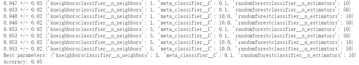
## 第一层不同的分类器可以适合训练数据集中的不同特征子集。
from sklearn.datasets import load_iris
from mlxtend.classifier import StackingCVClassifier
from mlxtend.feature_selection import ColumnSelector
from sklearn.pipeline import make_pipeline
from sklearn.linear_model import LogisticRegression

iris = load_iris()
X = iris.data
y = iris.target

pipe1 = make_pipeline(ColumnSelector(cols=(0, 2)), LogisticRegression())
pipe2 = make_pipeline(ColumnSelector(cols=(1, 2, 3)), LogisticRegression())

sclf = StackingCVClassifier(classifiers=[pipe1, pipe2],
                           meta_classifier=LogisticRegression(),
                           random_state=42)
sclf.fit(X, y)

——————

  • e. ROC曲线
1
2
3
4
5
6
7
8
9
10
11
12
13
14
15
16
17
18
19
20
21
22
23
24
25
26
27
28
29
30
31
32
33
34
35
36
37
38
39
40
41
42
43
44
45
46
47
48
49
50
51
52
53
from sklearn import model_selection
from sklearn.linear_model import LogisticRegression
from sklearn.neighbors import KNeighborsClassifier
from sklearn.svm import SVC
from sklearn.ensemble import RandomForestClassifier
from mlxtend.classifier import StackingCVClassifier
from sklearn.metrics import roc_curve, auc
from sklearn.model_selection import train_test_split
from sklearn import datasets
from sklearn.preprocessing import label_binarize
from sklearn.multiclass import OneVsRestClassifier

iris = datasets.load_iris()
X, y = iris.data[:, [0, 1]], iris.target

# Binarize the output
y = label_binarize(y, classes=[0, 1, 2])
n_classes = y.shape[1]
RANDOM_SEED = 42
X_train, X_test, y_train, y_test = train_test_split(X, y, test_size=0.33, random_state=RANDOM_SEED)

clf1 = LogisticRegression()
clf2 = RandomForestClassifier(random_state=RANDOM_SEED)
clf3 = SVC(random_state=RANDOM_SEED)
lr = LogisticRegression()
sclf = StackingCVClassifier(classifiers=[clf1, clf2, clf3], meta_classifier=lr)

# Learn to predict each class against the other
classifier = OneVsRestClassifier(sclf)
y_score = classifier.fit(X_train, y_train).decision_function(X_test)

# Compute ROC curve and ROC area for each class
fpr = dict()
tpr = dict()
roc_auc = dict()
for i in range(n_classes):
fpr[i], tpr[i], _ = roc_curve(y_test[:, i], y_score[:, i])
roc_auc[i] = auc(fpr[i], tpr[i])

# Compute micro-average ROC curve and ROC area
fpr["micro"], tpr["micro"], _ = roc_curve(y_test.ravel(), y_score.ravel())
roc_auc["micro"] = auc(fpr["micro"], tpr["micro"])
plt.figure()
lw = 2
plt.plot(fpr[2], tpr[2], color='darkorange', lw=lw, label='ROC curve (area = %0.2f)' % roc_auc[2])
plt.plot([0, 1], [0, 1], color='navy', lw=lw, linestyle='--')
plt.xlim([0.0, 1.0])
plt.ylim([0.0, 1.05])
plt.xlabel('False Positive Rate')
plt.ylabel('True Positive Rate')
plt.title('Receiver operating characteristic example')
plt.legend(loc="lower right")
plt.show()

输出:

2.3 Stacking与Blending的对比

Blending的优点在于比Stacking简单(不用使用K折交叉验证);缺点在于数据使用上有浪费(划分出了验证集),而且可能会过拟合(这里的原因大概率是数据使用少的问题)。

Stacking比Blending更加稳健(使用多次交叉验证)。

3 Stacking实战

  1. 幸福感预测,见Stacking集成学习案例一:幸福感预测
  2. 蒸汽量预测,见Stacking集成学习案例二:蒸汽量预测